The previous pages in this series looked at how accurate the data is: what it measures, what it is licensed for, how uncertain it is and how much that uncertainty moves the lines. All of them used the same code to turn the grid into lines. This page tests that code itself. If the tracer moves a line, it does not matter how accurate the model is.
I built a benchmark for the TopoLines tracer and ran it before changing anything. It found four issues. They are now fixed. This page shows how much each one affected the lines, how much has improved, and what remains to be done. The method for tracing contours is in the docs: how contours are traced.
The benchmark
Two types of terrain.
Synthetic terrain. A Gaussian hill, a saddle, a ridge and valley, wavy terrain, a steep noisy slope, a tilted plane, a closed basin 80 m below sea level, and a polder behind a dyke. Each is defined in metres and sampled on a grid laid out in degrees, like GEDTM30 and USGS 3DEP, at latitudes of 0°, 45°, 60° and 70°. As the exact position of every contour is known, this measures how much error comes from sampling the surface and tracing the contours. These tests run with the rest of the test suite on every change.
Six real zones, traced on GEDTM30 v1.2 (Ho et al., 2025) and, where one covers them, on the national lidar model: RGE ALTI from IGN in France, 3DEP in the United States.
| Zone | Box (W, S, E, N) | Size | Interval | Why |
|---|---|---|---|---|
| Calanques, Marseille | 5.38, 43.19, 5.48, 43.25 | 8.1 × 6.7 km | 25 m | Cliffs into the sea |
| Écrins, Barre des Écrins | 6.30, 44.89, 6.40, 44.95 | 7.9 × 6.7 km | 50 m | High mountain, steep |
| Camargue, Vaccarès | 4.50, 43.48, 4.60, 43.54 | 8.1 × 6.7 km | 5 m | Lagoon and land at 0 m |
| Badwater Basin, Death Valley | −116.82, 36.19, −116.72, 36.26 | 9.0 × 7.8 km | 25 m | Land 85 m below sea level |
| Zuidplaspolder, Netherlands | 4.55, 51.96, 4.67, 52.02 | 8.2 × 6.7 km | 5 m | Polder, flat, below 0 m |
| Girdwood, Alaska | −149.22, 60.93, −149.06, 60.99 | 8.7 × 6.7 km | 50 m | 61° N, sea arm |
To test the smoothing I added the Aiguille du Midi (6.86, 45.865, 6.91, 45.895), served by IGN at 2 m. That is where I had seen the raw trace wiggle.
I traced each zone at every simplification step and measured:
- Crossings: pairs of contours of different levels that touch or cross.
- Self-crossings: lines that cross themselves.
- Displacement: the Hausdorff distance in metres between the simplified line and the raw trace, and separately its east–west and north–south parts.
- Vertical error: the simplified line, sampled every half cell and read back on the grid. The simplification must never leave the band between the two neighbouring levels (Bayer et al., 2023): |dh| ≤ the interval. I also report the stricter half interval.
- Smoothing cost: the change in height on crests and valley floors (the 2 % of cells highest and lowest relative to their surroundings), the summits, the closed depressions, and how much of the line turns by more than 45° at a vertex (the cell-by-cell zig-zag).
Four defects
1. The tolerance was wider north–south
Simplification can move a line by up to the tolerance: 15 m at Medium. The code converted metres into degrees of longitude, then used the same number of degrees north–south. But a degree of longitude shrinks as latitude increases, so the north–south tolerance was the nominal value divided by cos(latitude).
On the synthetic terrain, the north–south / east–west ratio was 1.41 at 45°, 2.00 at 60° and 2.93 at 70°. At Girdwood (61° N), Medium displaced lines by up to 30.6 m north–south and 17.6 m east–west, for 15 m announced.
Now: the coordinates are scaled to metres before simplifying. Douglas–Peucker bounds the displacement by the tolerance, and the largest measured displacement reaches it in both directions on every zone: 15.0 m at Medium, from 36° N to 61° N.
2. Lines crossed at High
Douglas–Peucker simplifies one line at a time, without looking at the lines next to it. On a steep slope, a shortcut can cut across the next level. On the real zones this only happened at High: 18 crossing pairs in the Écrins (IGN 5 m), 18 at Badwater (3DEP), 5 in the Écrins (GEDTM30). On a synthetic 31° slope with 3 m of noise and a 5 m interval: 37 pairs at Low and 107 at Medium. Up to 9 lines also crossed themselves.
In a synthetic test, topology-preserving simplification applied one line at a time removed none of these crossings. The simplification has to consider all the lines together (Saalfeld, 1999).
Now: all the lines of a zone, contours and coastline, go into the topology-preserving simplifier of GEOS as a single multi-line geometry. It refuses any shortcut that would cross another segment of the collection. 0 crossings and 0 self-crossings on every zone and source, at every step. The cost: 0 to 3 % more points, and the step takes 4 to 6 times longer (indicative, one run per zone): 0.3 s at most on the benchmark zones, about 2 s for a trace of a million points.
3. Land below sea level was drawn as sea
Anything at 0 m or below was treated as sea. 51.9 % of Badwater was shown as sea, on both GEDTM30 and 3DEP, and no contour was drawn below 0 m: the lowest was +25 m on GEDTM30. 91.5 % of the Zuidplaspolder was sea, and 8 contours remained.
Looking at the raw grids, I expected the sea to be NoData. It is not. GEDTM30, IGN RGE ALTI and 3DEP all serve the sea as a flat surface at 0.0 m (the Calanques, the Turnagain Arm at Girdwood). In these models, open water is a large flat area with a single value, while land below sea level keeps measurable relief.
Now: a flat surface at sea level that reaches the open water is sea. Everything else is land, whatever its height. Badwater: 0 % sea, contours at −25, −50 and −75 m (the floor is at −85 m). Polder: 0 % sea, 253 contours down to −10 m, 102 of them closed depressions. The Calanques and Girdwood keep their sea exactly as before.
Depressions are now found from the direction of the ring: marching squares always leaves the lower ground on the same side of the line. Compared with the previous method, on 781 closed rings from the real zones, the two disagreed on 55. All were small rings, and every one large enough to sample has lower ground inside.
4. Smoothing flattened the relief on GEDTM30
Before tracing, the grid is smoothed to reduce its noise (Fisher & Tate, 2006), which marching squares would otherwise draw as a zig-zag. The smoothing was 2 cells wide: 10 m on a 5 m lidar grid, but 45 to 60 m on GEDTM30. And GEDTM30 has already been smoothed by its authors, with an adaptive and a bilateral filter (Ho et al., 2025). The grid was smoothed twice.
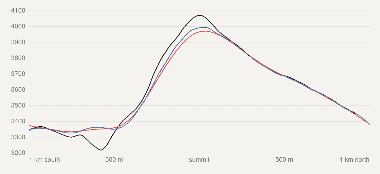
On the five mountain zones on GEDTM30, the crests were lowered by 15 to 31 m on average and the valley floors filled by 12 to 26 m. The closed depressions were lost: 3 left of 75 at Girdwood. Between 0.14 and 15.6 % of the raw trace ended up more than half an interval away from the published grid; with a 25 m interval, that is 12.5 m.
Now: the smoothing is set in metres, the same in every direction, and follows the cell size of the grid being served. GEDTM30 is smoothed by a fraction of a cell. Raw national lidar is smoothed more, enough to remove its grid noise.
| GEDTM30, before → now | Crests (m) | Valley floors (m) | Depressions: grid / before / now | Raw trace beyond ½ interval |
|---|---|---|---|---|
| Calanques | −23.4 → −2.0 | +20.5 → +1.9 | 14 / 0 / 7 | 14.0 → 0.01 % |
| Écrins | −31.1 → −2.6 | +25.6 → +2.6 | 11 / 0 / 4 | 3.5 → 0.00 % |
| Badwater | −19.1 → −1.8 | +20.6 → +1.9 | 3 / 0 / 0 | 11.2 → 0.00 % |
| Girdwood | −15.5 → −1.0 | +12.4 → +1.0 | 75 / 3 / 37 | 0.14 → 0.00 % |
| Aiguille du Midi | −25.2 → −2.3 | +21.3 → +2.9 | 4 / 0 / 1 | 15.6 → 0.00 % |
The lines now show more of the real relief, so they hold more points: 33 to 75 % more at Medium.
The wobble is real
On the Aiguille du Midi (2 m), the raw lidar trace turned by more than 45° at 24 % of its vertices: marching squares drawing the grid noise as a zig-zag. After the lidar smoothing, 0.01 %. What I saw as a wiggling line is real: rocks, scree and small rock steps a few metres across, which are in the model. Widening the smoothing to 10 m barely changed the line, and it took 2.5 m off the crests. So I left the smoothing as it was and added a simplification step instead: Fine · 2 m.
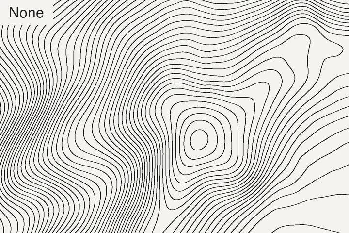
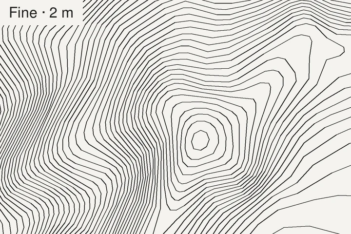
On 5 m lidar, Fine · 2 m removes 85 to 93 % of the points, and no line moves by more than 2.0 m. The vertical error never goes beyond the interval. A grid with 5 m cells holds no detail smaller than 2 m, so a 2 m step removes nothing real.
What was tried and dropped
- One smoothing width in metres for every grid. 10 m left too much noise on GEDTM30; 15 m took 5 to 6 m off the crests on lidar. The noise is at the scale of each grid’s cell, so the smoothing has to follow the cell size.
- A blend of light and strong smoothing, weighted by how much each cell stands out from its surroundings (Kettunen et al., 2017). The paper describes the method but gives no parameter values, so I calibrated them on the benchmark. On relief it produced the same lines as the current rule, but took 7 times longer. On the polder it left 436 to 827 small loops depending on the threshold, still far from the 103 before. On the Camargue it either drew a contour more than half an interval away from the data along its whole length, or lost the two real ones. Not kept. The last step of the same paper, removing contours that are too short, was kept: it is the Auto option of Min. contour length.
- A smoothing that preserves breaks in slope (Lindsay et al., 2019). It kept the lidar crests within 1 m and every depression, but also the grid zig-zag: 2.9 % of sharp turns in the Écrins, against 0.01 % with the current smoothing. That is intended, since it helps drainage analysis. Not kept for contours.
What is still open
- Flat ground on GEDTM30 is busier. With less smoothing, the polder at a 5 m interval has 1,294 small closed loops around decimetres of relief, against 103 before. They are in the data: the previous lines were more than half an interval away from the grid on 6 % of their length. Auto minimum length brings them down to 360 and keeps 80 % of the length.
- The Camargue is not settled. The lagoon is served as a flat area just below 0 m, next to land that is also just below 0 m. Without a water mask to refer to, the benchmark cannot tell them apart everywhere. This is a limit of any method that reads elevation alone: flat water looks the same as flat land at the same height. Only a separate water mask can settle it.
- The OpenStreetMap coastline was not tested on real zones. The coastline server did not answer in time during the measurements, so every coastal zone was cut along the model’s own sea surface. The OSM path is only covered by a synthetic test.
- Saddles are resolved with one fixed rule. Not measured as a problem on these zones.
- Coarser grids for large lidar zones are resampled by the provider’s service, or bilinearly, with no low-pass filter first. Not measured.
- The data is still the biggest source of error. At the Écrins summit the tracer now costs 1.4 m, where GEDTM30 itself is 75 m below the lidar. A vertical error h moves a contour by h / tan θ on a slope θ; Miller (2024) uses the same relation to bound how far a smoothed line may move. The previous page measured it.
Method
- Data: GEDTM30 v1.2 by OpenGeoHub (Ho & Hengl, 2026), read from OpenTopography, CC BY 4.0. IGN RGE ALTI at 5 m (2 m on the Aiguille du Midi), Etalab Open Licence 2.0. USGS 3DEP sampled at 5 m, public domain. Grids as served to the app, on 15 November 2026. The 3DEP grid is not square on the ground: 5.0 × 6.2 m at Badwater, 5.0 × 10.3 m at Girdwood.
- Code: the measurement script calls the tracer’s own functions, in the same order as in production, with the trace cache switched off. Nothing is rewritten. Marching squares from scikit-image 0.25.2 (van der Walt et al., 2014), geometry from Shapely 2.1.2 on GEOS 3.13.1, Python 3.12.
- Distances in metres use a local scale at the zone’s median latitude, as the tracer does. On zones up to 45 km across, this is within ±0.35 % of a projected distance.
- Vertical error is read on the smoothed grid when judging the simplification, and on the published grid when judging the smoothing.
- Smoothing variants were each applied to the same raw grid, then traced by the same chain.
- One run per zone. Total trace times depend on the network and are not compared. The simplification times are local computation only, and indicative.
- Figures on this page come from the same raw grids and the same code.
Thank you to the people who make this possible to test: OpenGeoHub, for publishing GEDTM30 and how it was made; IGN and the U.S. Geological Survey, for publishing their lidar terrain openly; and the authors of the papers above, for describing their methods in enough detail to be tested.
What TopoLines uses
Everything above is live since Beta v2.56.0: tolerance in ground metres, all lines simplified together, land below 0 m traced, depressions by orientation, smoothing that follows the cell of the grid served, the Fine · 2 m step, and Recommended and Auto in the Settings panel. The full method is in the docs: how contours are traced.
References
- Bayer, T., Kolingerová, I., Čelonk, M. & Lysák, J. (2023). Simplification of contour lines, based on axial splines, with high-quality results. International Journal of Geographical Information Science 37(7), 1520–1554. doi:10.1080/13658816.2023.2193969
- Miller, S. (2024). Locally adjusted curve approximation smoothing of contour polylines. Journal of Spatial Information Science 28, 3–73. doi:10.5311/josis.2024.28.245
- Douglas, D. H. & Peucker, T. K. (1973). Algorithms for the reduction of the number of points required to represent a digitized line or its caricature. Cartographica 10(2), 112–122. doi:10.3138/fm57-6770-u75u-7727
- Saalfeld, A. (1999). Topologically consistent line simplification with the Douglas-Peucker algorithm. Cartography and Geographic Information Science 26(1), 7–18. doi:10.1559/152304099782424901
- Fisher, P. F. & Tate, N. J. (2006). Causes and consequences of error in digital elevation models. Progress in Physical Geography 30(4), 467–489. doi:10.1191/0309133306pp492ra
- Ho, Y.-F., Grohmann, C. H., Lindsay, J., Reuter, H. I., Parente, L., Witjes, M. & Hengl, T. (2025). GEDTM30: global ensemble digital terrain model at 30 m and derived multiscale terrain variables. PeerJ 13, e19673. doi:10.7717/peerj.19673
- Ho, Y. & Hengl, T. (2026). Global Ensemble Digital Terrain Model 30m (GEDTM30), v1.2.0. Zenodo. doi:10.5281/zenodo.18887460
- Kettunen, P., Koski, C. & Oksanen, J. (2017). A design of contour generation for topographic maps with adaptive DEM smoothing. International Journal of Cartography 3(1), 19–30. doi:10.1080/23729333.2017.1300998
- Lindsay, J. B., Francioni, A. & Cockburn, J. M. H. (2019). LiDAR DEM smoothing and the preservation of drainage features. Remote Sensing 11(16), 1926. doi:10.3390/rs11161926
- van der Walt, S., Schönberger, J. L., Nunez-Iglesias, J., Boulogne, F., Warner, J. D., Yager, N., Gouillart, E., Yu, T. & the scikit-image contributors (2014). scikit-image: image processing in Python. PeerJ 2, e453. doi:10.7717/peerj.453
- IGN (2026). RGE ALTI®. cartes.gouv.fr.
- U.S. Geological Survey (2026). 3D Elevation Program. usgs.gov.
Last updated 15 November 2026