Every elevation model has an accuracy figure: one number, an RMSE, measured somewhere and averaged over the world. But a contour line runs through particular ground, in a particular wood, on a particular slope, and the error there can be much smaller or much larger than the average. This page is the third in a short series on when a contour line can be trusted; the first was about what the data measured, the second about what you may do with it.
GEDTM30, the open terrain model by OpenGeoHub, does something most models don’t: next to each 30 m terrain height it publishes a second number, the model’s own uncertainty about that height. We mapped it under real contours and checked it against airborne lidar.
One number per cell
GEDTM30 was built with a random forest, a machine-learning model made of many decision trees, trained on almost 30 billion ground heights from two satellite lidars, ICESat-2 and GEDI. A global forest of 100 trees was refined, tile by tile where there were enough local samples, with 100 more trees trained on them. The published height is the mean of all the trees’ predictions, then filtered to remove speckle. The uncertainty layer is their standard deviation: how much the trees disagree about that cell (Ho et al., 2025). This page calls it σ.
Yu-Feng Ho, GEDTM30’s first author, explained the difference this makes in his 2026 OpenGeoHub Summer School lecture on uncertainty. A model faces two kinds of uncertainty: what the model itself doesn’t know, called epistemic (8:07), and the noise already present in the training data, called aleatoric (8:47). More samples or a better model can reduce the first, not the second (9:19). In a random forest, how much the trees differ from each other measures the first kind, the model’s uncertainty (18:35). So σ says where the model is unsure. It is not, by construction, the full error.
Across the world, σ is highest in dense forests such as the Amazon and the Congo basin and in the great mountain ranges, the Himalayas, the Andes and the Alps; the authors find it tied to steepness and canopy density, in line with earlier studies of terrain model error. It is also high over some water bodies and parts of Greenland, which they put down to the inputs rather than the land: optical satellite layers that represent water poorly, and layers that do not exist for Greenland at all (Ho et al., 2025, Fig. 13).
What σ looks like under contours
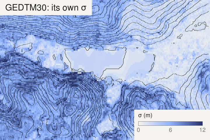
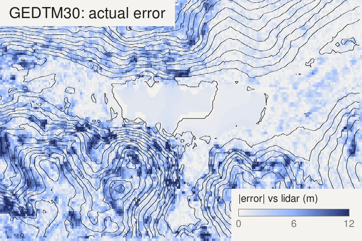
The two maps agree on the broad picture. Over the lake, the meadows and the flat valley floor, σ is 3 m or less and the real error about 1 m. On the wooded slopes around them, σ rises to 7 m and the real error to 3 or 4 m. Cell by cell, the match is looser: σ is a smooth field, while the real error comes in spots, a bad cell next to a good one. Over this frame the correlation between the two is 0.5. σ tells you which parts of a map to doubt, not which cell is wrong.
From a height to a band on the map
A vertical uncertainty becomes a horizontal one on the map. On a slope of angle θ, a height off by σ moves its contour sideways by σ / tan θ, the same rule as for the tree-top lift in the first page. So for each contour you can shade the strip where the line would run if the error were one σ either way: the cells where the contour’s level lies between the height minus σ and the height plus σ.
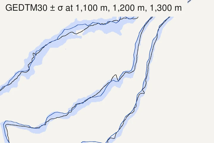
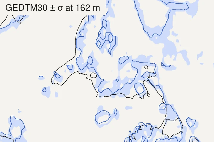
The two frames say opposite things. On the steep slope, σ is ten times larger than on the flat ground, but the band is not wider: over each frame, the median half-width of the band is about 30 m on the slope and about 40 m on the flat. A large σ on steep ground is harmless to a contour’s position; a small σ on flat ground is not. And on the flat, the real line leaves the band, which means σ there was too small; the next section measures how often.
A band only covers what the grid can show. Uncertainty and resolution are two different things: a bank, a small gully or a sharp break of slope narrower than a 30 m cell is not in the model at all, so no band will hint at it.
Does σ match the real error?
If σ were a standard deviation in the textbook sense, of an error spread like a bell curve, about 68% of cells would fall within ±σ of the truth and 95% within ±2σ. In his lecture, Ho warns that a random forest’s predictions need not follow a bell curve, which makes a standard deviation risky to read (43:42). So we measured it, against the IGN LiDAR HD ground at four sites:
| Site | Cells | Median σ | Median real error | RMSE | Within ±σ | Within ±2σ |
|---|---|---|---|---|---|---|
| Lac de Gérardmer (Vosges), lake and woods | 21,364 | 5.7 m | 1.9 m | 4.0 m | 87% | 99% |
| Chamonix valley (Haute-Savoie), mountain | 13,026 | 8.9 m | 2.9 m | 7.0 m | 88% | 98% |
| Central Vercors (Drôme), plateau and slopes | 8,905 | 6.2 m | 2.1 m | 4.4 m | 90% | 99% |
| Rambouillet forest edge (Yvelines), flat | 21,560 | 2.2 m | 1.6 m | 4.0 m | 52% | 83% |
In hills and mountains, σ is cautious: close to nine cells in ten fall within ±σ, far more than the 68% a bell curve would give, and almost all within ±2σ. There, reading σ as a safe margin works.
On the flat Rambouillet ground, σ is too optimistic: only half the cells are within ±σ. On its open fields, where σ is about 1 m, the share drops to 42%. Part of that gap is a constant offset of about 1 m between GEDTM30 and the lidar over the site, which may come partly from the two height references (EGM2008 for GEDTM30, NGF-IGN69 for the lidar). Removing the median offset (of all cells, or of the fields alone) raises the share within ±σ to 61% overall and 74% on the fields: better, but still below the hills. Where the land is flat, σ is small because the trees agree, and they can agree on the wrong height.
Two of the patterns the paper describes show up here too. σ follows the slope (correlation 0.57 to 0.66 at the three hilly sites) and the tree cover (0.45 to 0.65 at all four).
An offset or a spread
An error can be the same across a whole map, or it can vary from cell to cell, and the two do very different things to contours. An offset shared by a whole sheet moves every line by the same height: the numbers on the lines are off, but their shapes, the spacing and the landforms are not. An error that varies from cell to cell bends the lines themselves.
The paper’s global check against GNSS stations shows both at once. Against those stations, GEDTM30 had the lowest errors of the terrain models tested (against reference lidar terrain models, FathomDEM did best): a mean error of 7.34 m, a standard deviation of 7.77 m and an RMSE of 10.69 m (Ho et al., 2025, Fig. 12). Since 7.34² + 7.77² ≈ 10.69², the squared error splits about evenly between a common offset and a spread. The authors note that systematic gaps between satellite terrain models and GNSS heights persist, as an earlier validation had reported (Ince et al., 2024). At our four lidar sites, the offset was much smaller, within about 1 m, and the error was mostly spread: that is the part σ tries to describe, and the part that moves contours.
How to use σ on your own map
- Get the layer. The 30 m σ layer is a cloud-optimised GeoTIFF listed on GEDTM30’s Zenodo record, beside the terrain itself (the record’s own files are at 240 m). QGIS can open it straight from its URL as a raster layer. Its values are stored in metres: the record’s layer table gives a scale of 1, but the file carries a 0.1 scale tag, so if your software shows σ under a metre on a mountainside, it has applied the tag.
- Read σ against your contour interval. Where σ is larger than the interval, two neighbouring lines can each be off by more than the gap between them: their order holds better than their exact position. For choosing the interval itself, see choosing a contour interval.
- Read σ against the slope. Divide it by the tangent of the slope to get how far the line can move sideways. On gentle ground a small σ still means a wide band.
- Trust σ more in relief than on the flat. In our tests σ was a cautious margin in hills and mountains, and an optimistic one on flat ground.
- Where it matters, compare with a lidar terrain model. σ is the model judging itself; a national lidar model, where there is one, is an outside check.
How we measured
- Data: GEDTM30 v1.2 terrain and σ, read from OpenGeoHub’s 30 m files (Zenodo record); IGN’s LiDAR HD MNT (ground) and MNS (surface), read at 2 m (3 m for the Gérardmer lake frame) through IGN’s WMS-R service (IGN, LiDAR HD).
- Comparison: on GEDTM30’s own 30 m grid, with the lidar ground averaged into each cell. Real error = GEDTM30 minus lidar ground. Slope = from the lidar ground at 30 m. Wooded and open cells, in the text, are those more than 80% and less than 10% covered by objects over 5 m (lidar surface minus ground). Heights are compared as published, EGM2008 for GEDTM30 and NGF-IGN69 for the lidar; the offset-removed shares in the text subtract each site’s median difference.
- Bands: GEDTM30 and σ interpolated bilinearly to a finer grid, band = where the level lies within σ of the height. The lidar ground was smoothed over about 6 m before tracing.
- Contours are traced with the same marching-squares code as TopoLines’ exports.
- Limits: four sites in France, all with lidar; they say how σ behaved there, not everywhere. The lidar and GEDTM30’s inputs date from different years.
Credit: this page follows Yu-Feng Ho’s work, the uncertainty map of the GEDTM30 paper (Ho et al., 2025) and his lecture on uncertainty quantification at the OpenGeoHub Summer School 2026. The data are GEDTM30 v1.2 by Ho & Hengl, OpenGeoHub, CC BY 4.0 (doi.org/10.5281/zenodo.18887460), from which we traced the contours and computed the comparisons, and LiDAR HD © IGN, Etalab 2.0 (data.gouv.fr/datasets/mnt-lidar-hd).
What TopoLines uses
TopoLines traces GEDTM30 by default, but does not read its σ layer: the exported contours are traced from the terrain heights alone. To see how sure the model is of the ground under your map, open the σ layer beside it, as above.
Publishing σ costs a model’s makers something: it shows, cell by cell, where their work is weakest. OpenGeoHub chose to publish it anyway, openly, for everyone. A single accuracy figure could not have told us any of the above.
References
- Ho, Y.-F., Grohmann, C. H., Lindsay, J., Reuter, H. I., Parente, L., Witjes, M. & Hengl, T. (2025). GEDTM30: global ensemble digital terrain model at 30 m and derived multiscale terrain variables. PeerJ 13, e19673. doi:10.7717/peerj.19673
- Ho, Y. & Hengl, T. (2026). Global Ensemble Digital Terrain Model 30m (GEDTM30), v1.2.0. Zenodo. doi:10.5281/zenodo.18887460
- Ho, Y.-F. (2026). Machine learning models with uncertainty quantification. OpenGeoHub Earth Observation Summer School 2026, Istanbul (recorded talk).
- Ince, E. S., Abrykosov, O. & Förste, C. (2024). GDEMM2024: global digital elevation merged model 2024 for surface, bedrock, ice thickness, and land-type masks. Scientific Data 11, 1087. doi:10.1038/s41597-024-03920-x
- IGN (2026). MNT LiDAR HD. data.gouv.fr.
Last updated 11 November 2026