10 classic mistakes with elevation data

Surface instead of terrain, feet read as metres, geoid vs ellipsoid, contours in degrees, hidden vertical exaggeration and five more: how each one shows up in your map, and how to catch it before it ships.

Every figure and link on this page was checked against its source (the publisher's documentation, a standard or a peer-reviewed paper) on 5 November 2026. Spotted something out of date? Tell us on GitHub.

Most elevation mistakes don’t crash anything. They produce a map that looks perfectly reasonable and is wrong. These ten are the ones that come up again and again on GIS forums, each with the symptom to look for and the check that catches it.

1. Contouring a surface model

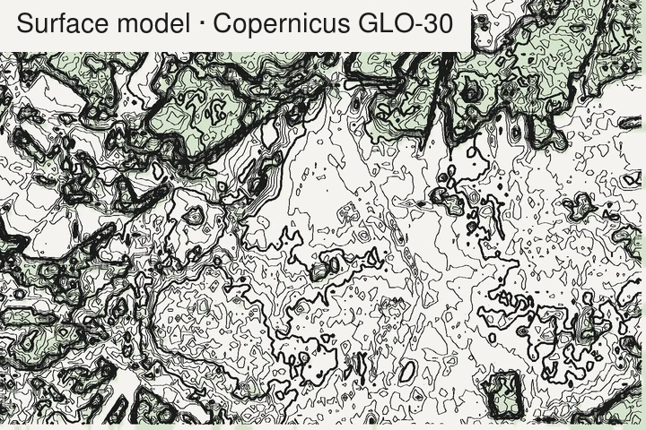
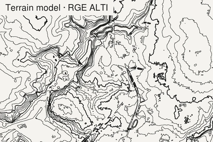
Symptom: contours wiggle around every wood, draw rectangles in towns, and a forested ridge comes out several metres, sometimes tens of metres, higher than the map says.

Why: the dataset is a DSM (surface: tree tops, roofs), not a DTM (bare ground); the terms are defined in Guth et al. (2021). Copernicus GLO-30, SRTM and NASADEM, ALOS AW3D30, ArcticDEM and REMA are all surface models.

Check: look up the product type before downloading. On a forest edge, a surface model shows a step the height of the trees. See which global models are bare earth.

Contours every 2 m from Copernicus GLO-30: tight bundles around every wood — The same 4.5 × 3 km at the edge of the Rambouillet forest (Yvelines), contoured every 2 m. Left: Copernicus GLO-30, a surface model; green marks where it stands more than 5 m above the RGE ALTI ground, i.e. trees and roofs. Right: RGE ALTI, bare ground, showing the valley the woods hide.

Contours every 2 m from RGE ALTI: a smooth valley and plateau — The same 4.5 × 3 km at the edge of the Rambouillet forest (Yvelines), contoured every 2 m. Left: Copernicus GLO-30, a surface model; green marks where it stands more than 5 m above the RGE ALTI ground, i.e. trees and roofs. Right: RGE ALTI, bare ground, showing the valley the woods hide.

2. Feet read as metres (or the reverse)

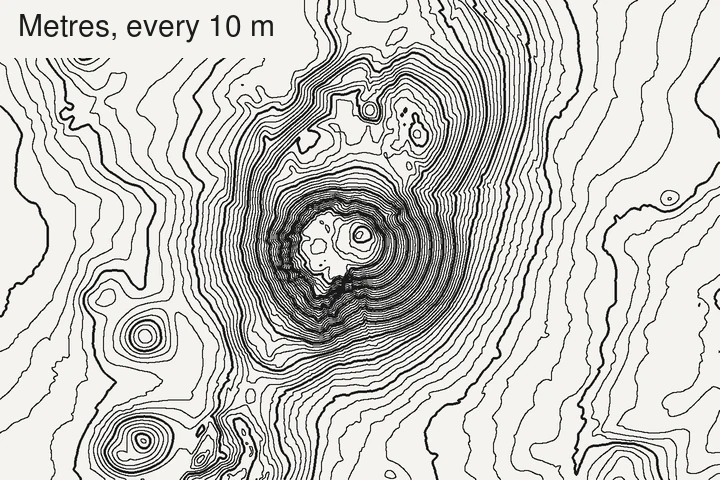
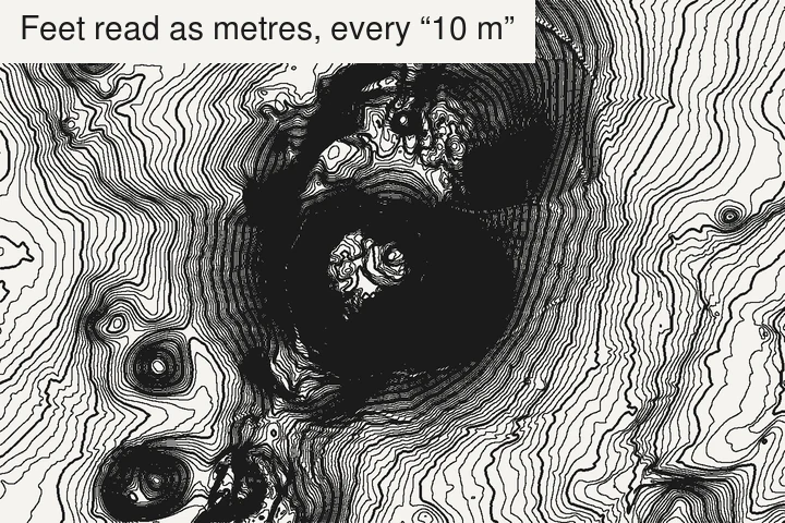
Symptom: a “10 m” interval gives three times too many lines, or a mountain stands at 4,000 m when it should be 1,200.

Why: a lot of US lidar and state data is in US survey feet. Nothing in the pixel values says so.

Check: read the vertical unit in the metadata (gdalinfo shows it if the file declares it). Then sanity-check one known point, such as a summit, against a map.

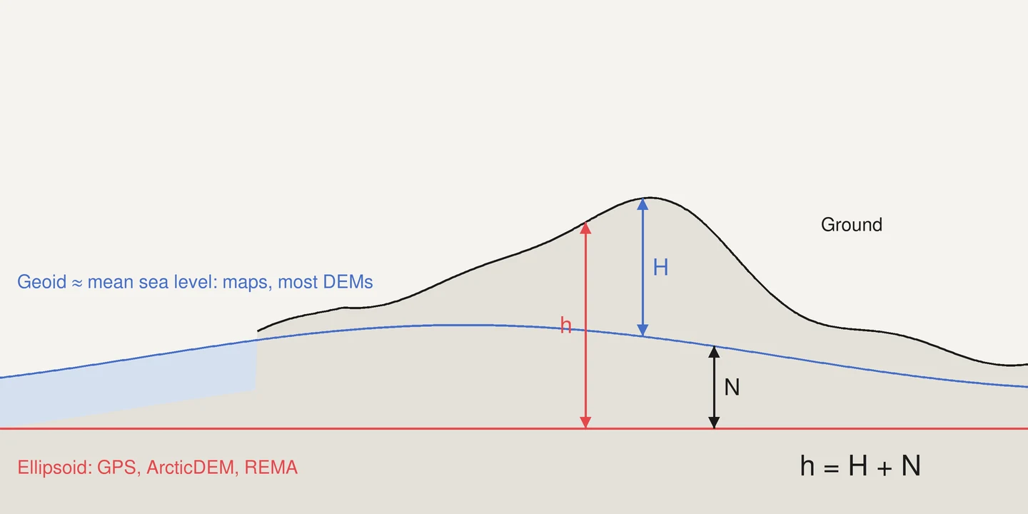
Puy de Dôme contoured every 10 m from heights in metres — Puy de Dôme, RGE ALTI, contoured every 10 m. Right: the same grid converted to feet and read as metres, so 3.28 times as many lines.

The same area with heights in feet read as metres: lines 3.28 times denser — Puy de Dôme, RGE ALTI, contoured every 10 m. Right: the same grid converted to feet and read as metres, so 3.28 times as many lines.

3. Mixing geoid and ellipsoid heights

Symptom: your GPS track floats above the terrain, or sinks into it, by a constant tens of metres. Coastal pixels show negative heights.

Why: GPS and some datasets (ArcticDEM, REMA) give heights above the ellipsoid; maps and most DEMs give heights above the geoid (roughly, mean sea level). The gap, the geoid height, ranges from about −107 m (in the Indian Ocean, south of India) to about +86 m (New Guinea) in the EGM2008 model (Pavlis et al., 2012); across mainland France it’s between about 42 and 56 m.

Check: confirm the vertical CRS of every layer, and convert with a geoid grid (PROJ and QGIS handle it when the vertical CRS is set) before comparing.

Diagram: ground, geoid and ellipsoid, with h, H and N — Schematic, not to scale. h: height above the ellipsoid (GPS). H: height above the geoid (maps, most DEMs). N: the geoid height between them, about −107 m to +86 m worldwide in EGM2008.

4. Contouring in degrees

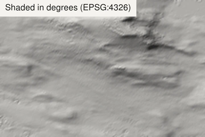
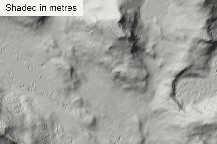
Symptom: smoothing and minimum-length settings behave differently north–south and east–west; slope and hillshade look stretched.

Why: the raster is in geographic coordinates (EPSG:4326), where one degree of longitude shrinks with latitude.

Check: reproject to a metric projection (UTM, or the national one: Lambert-93, British National Grid…) before contouring, slopes or hillshades.

Hillshade of a grid in degrees shown with square cells: relief stretched east–west — Jotunheimen, Norway (61.5° N), GEDTM30. At this latitude a one-arcsecond cell is about 15 m wide and 31 m tall on the ground. Left: the grid shaded and displayed as if its cells were square (central part of the area), so the relief is stretched east–west and slopes are misread. Right: the same data with its true cell sizes.

Hillshade of the same grid with its true cell sizes — Jotunheimen, Norway (61.5° N), GEDTM30. At this latitude a one-arcsecond cell is about 15 m wide and 31 m tall on the ground. Left: the grid shaded and displayed as if its cells were square (central part of the area), so the relief is stretched east–west and slopes are misread. Right: the same data with its true cell sizes.

5. Hidden vertical exaggeration

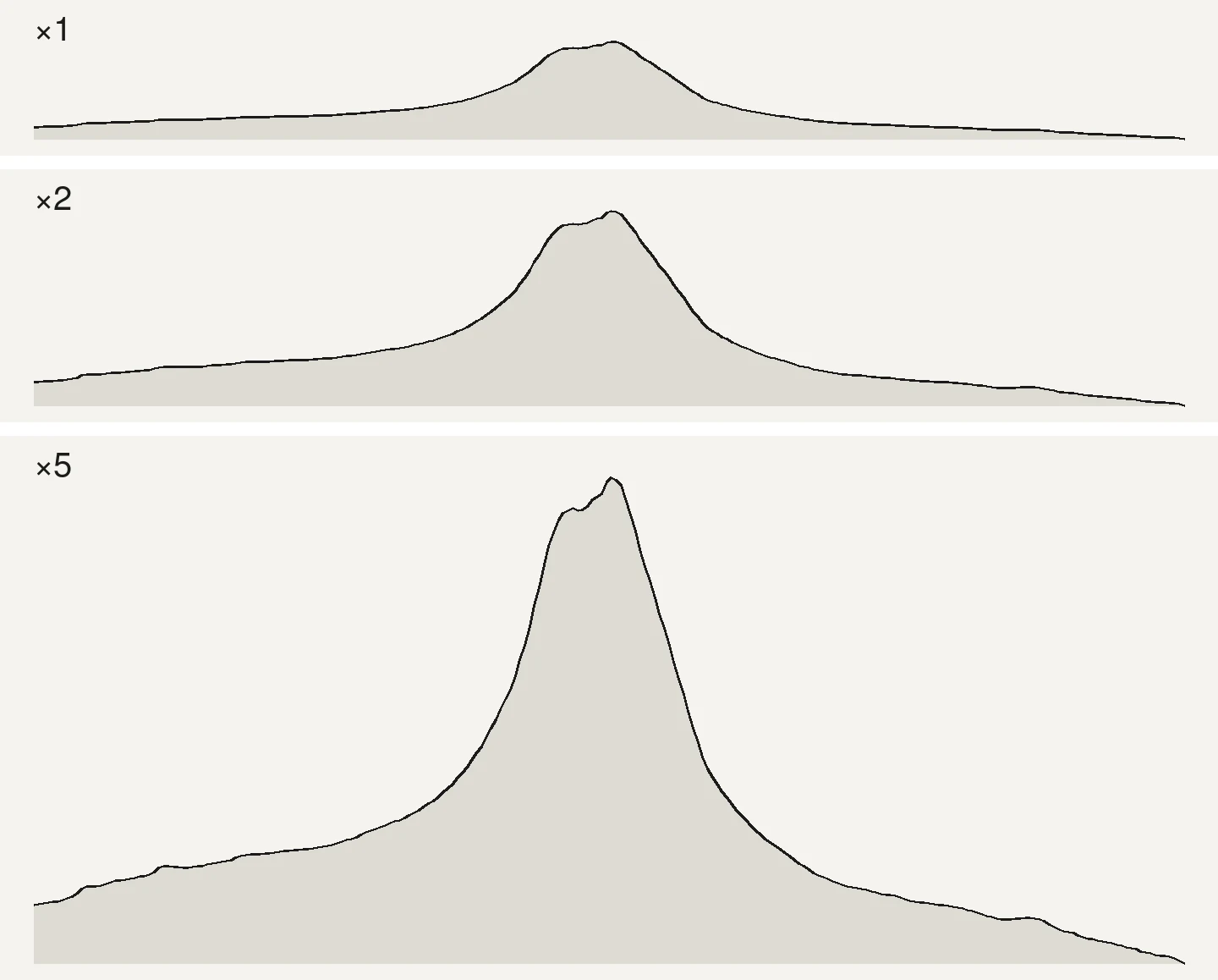
Symptom: a 3D render or a terrain profile makes rolling hills look like the Himalaya, and nobody can tell by how much.

Why: exaggeration is often set to make a render “read”, then never mentioned.

Check: state the factor next to the image (×1, ×2…). For profiles, give both axes the same units and say the ratio.

One real profile, 8 km west to east through the Puy de Dôme (RGE ALTI), drawn three times. Only ×1 shows the true shape.

6. Tile seams and NoData edges

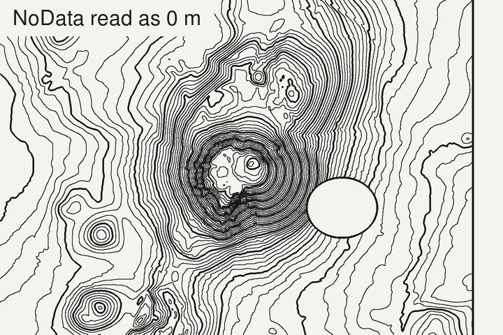
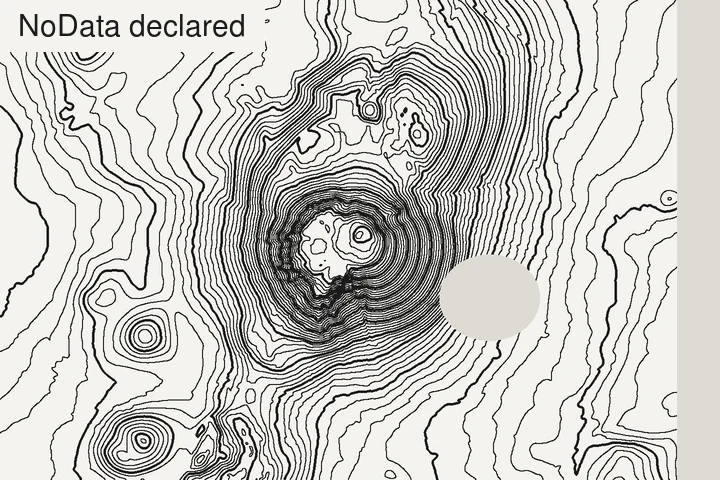
Symptom: straight lines in the contours along a grid, cliffs at tile boundaries, or contour rings around holes.

Why: tiles from different flights or years don’t match exactly, and NoData cells at the edges get read as 0 m or as a wall.

Check: mosaic first (a VRT is enough), make sure NoData is declared, and fill small voids before contouring.

Contours with a void read as 0 m: a black ring and a wall along the edge — Puy de Dôme, every 10 m, with a void and a strip of missing cells along the edge (cut into the real grid for this figure). Left: missing cells read as 0 m, so every level from 0 m up piles into a black ring around the hole and a wall along the edge. Right: NoData declared, so the contours stop at the void.

The same contours with the void declared as NoData, shown grey — Puy de Dôme, every 10 m, with a void and a strip of missing cells along the edge (cut into the real grid for this figure). Left: missing cells read as 0 m, so every level from 0 m up piles into a black ring around the hole and a wall along the edge. Right: NoData declared, so the contours stop at the void.

7. Resampling with nearest neighbour

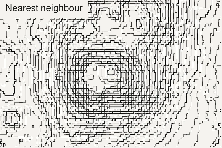
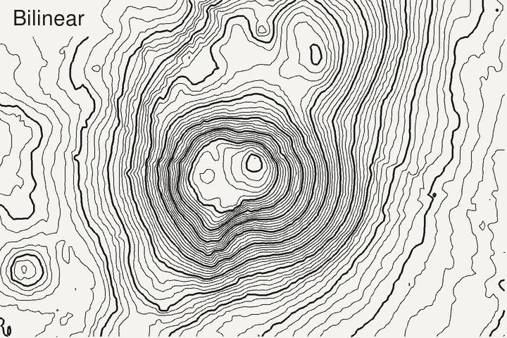
Symptom: staircase contours, small terraces on smooth slopes.

Why: reprojecting or resizing an elevation raster with nearest neighbour copies cells in blocks.

Check: use bilinear or cubic resampling for continuous data like elevation. Keep nearest neighbour for categories (land cover).

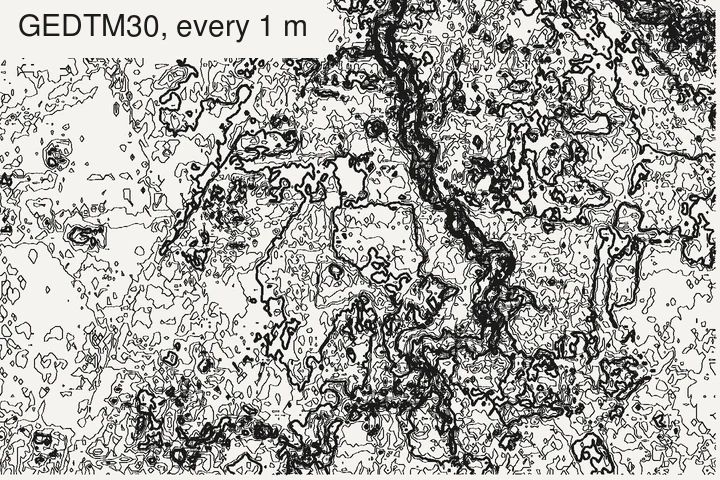
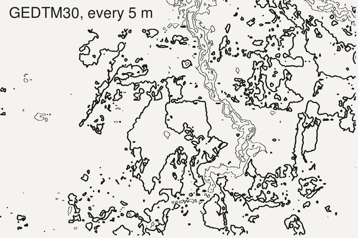
Staircase contours from a nearest-neighbour upsampled DEM — GEDTM30 around the Puy de Dôme brought from 30 m to a 5 m grid, contoured every 10 m. Nearest neighbour copies each 30 m cell as a block (left); bilinear interpolates between cells (right).

Smooth contours from the same DEM upsampled bilinearly — GEDTM30 around the Puy de Dôme brought from 30 m to a 5 m grid, contoured every 10 m. Nearest neighbour copies each 30 m cell as a block (left); bilinear interpolates between cells (right).

8. An interval finer than the data

Symptom: a maze of tiny closed loops on flat ground.

Why: the interval is smaller than the data’s vertical noise, so the contours trace the noise.

Check: keep the interval at about 3.3 times the data’s vertical RMSE, the equivalent of the 1947 National Map Accuracy Standards rule (90% of heights within half an interval). On flat, low-lying ground, global 30 m models are at their weakest (Guth et al., 2024): use lidar or a larger interval. How to choose an interval.

Flat ground contoured every 1 m: a maze of tiny loops — Flat Landes ground (27 m of relief over 6 × 4 km), GEDTM30. Every 1 m, the lines follow the model's noise as much as the ground (left); every 5 m, only the real shapes remain (right).

The same ground every 5 m: a few clean lines — Flat Landes ground (27 m of relief over 6 × 4 km), GEDTM30. Every 1 m, the lines follow the model's noise as much as the ground (left); every 5 m, only the real shapes remain (right).

9. Trusting the grid size as the level of detail

Symptom: a 1 m DEM that still looks smooth, or misses a 3 m wide ditch.

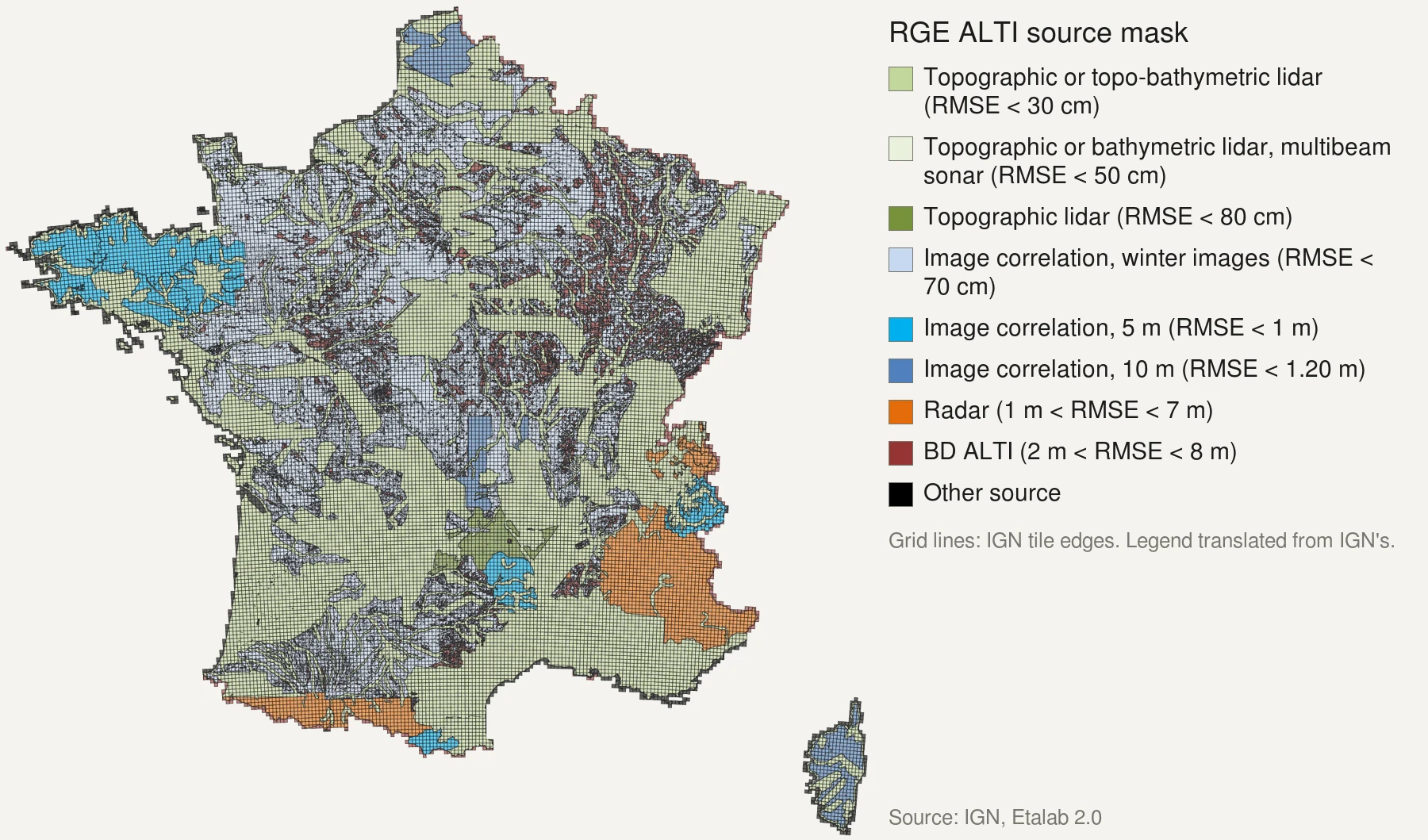
Why: a grid can be resampled from coarser sources. France’s RGE ALTI is a 1 m grid across the country, but built from radar in the high Alps and the Pyrenees, with errors around 7 m on steep slopes; global 30 m models are often smoother than 30 m.

Check: read which source covers your area, not just the pixel size. France’s patchwork, explained.

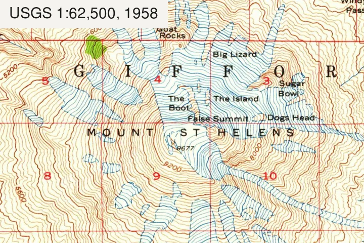
Map of mainland France and Corsica coloured by the source of each part of RGE ALTI: lidar, image correlation, radar, BD ALTI — RGE ALTI is a 1 m grid everywhere, but IGN's source mask shows what is under it: lidar, image correlation, radar or the old BD ALTI.

10. Old data presented as current

Symptom: a quarry, a new road or a landslide is missing, or a filled-in pit is still there.

Why: SRTM is from 2000, Copernicus from 2011–2015, and national lidar from the year it was flown.

Check: put the acquisition date of the data in the map’s credits, next to the source.

USGS 1958 map of Mount St. Helens with its summit at 9,677 ft — Mount St. Helens on two USGS maps, same 5.4 × 3.6 km. 1958 (left): the summit at 9,677 ft. 1983 (right): the 1980 crater and its lava dome. Any elevation data acquired before the May 1980 eruption still shows the left one. Scans: USGS Historical Topographic Map Collection, public domain.

USGS 1983 map of the same area showing the 1980 crater and lava dome — Mount St. Helens on two USGS maps, same 5.4 × 3.6 km. 1958 (left): the summit at 9,677 ft. 1983 (right): the 1980 crater and its lava dome. Any elevation data acquired before the May 1980 eruption still shows the left one. Scans: USGS Historical Topographic Map Collection, public domain.

References

Guth, P. L., Van Niekerk, A., Grohmann, C. H., Muller, J.-P., Hawker, L., Florinsky, I. V., Gesch, D., Reuter, H. I. et al. (2021). Digital elevation models: terminology and definitions. Remote Sensing 13(18), 3581. doi:10.3390/rs13183581
Pavlis, N. K., Holmes, S. A., Kenyon, S. C. & Factor, J. K. (2012). The development and evaluation of the Earth Gravitational Model 2008 (EGM2008). Journal of Geophysical Research: Solid Earth 117(B4). doi:10.1029/2011JB008916
Guth, P. L., Trevisani, S., Grohmann, C. H., Lindsay, J., Gesch, D., Hawker, L. & Bielski, C. (2024). Ranking of 10 global one-arc-second DEMs reveals limitations in terrain morphology representation. Remote Sensing 16(17), 3273. doi:10.3390/rs16173273
U.S. Bureau of the Budget (1947). United States National Map Accuracy Standards. reproduced in USGS, Map Accuracy (National Mapping Program fact sheet).

Last updated 5 November 2026