TopoLines draws contour lines from open elevation models. They are accurate enough for a lot of work, and not for some of it. This page says where the line is.
Good for
- Design, illustration, posters, laser cutting and 3D printing.
- Reading and presenting the shape of a site, a valley or a route.
- Early-stage planning and concept work: massing studies, site context, landscape sketches.
- Teaching and explaining terrain.
Not for
- Property boundaries, setbacks or any legal description of land.
- Permit drawings, construction or engineering design, including grading, drainage and cut-and-fill volumes.
- Flood, landslide or other risk decisions.
- Navigation where safety depends on it. Carry an official map.
For any of these, you need a survey by a licensed land surveyor (a géomètre-expert in France, a licensed surveyor in the US or UK). A disclaimer on a drawing does not make derived contours fit for these uses.
How the contours are made
Every trace goes through the same steps, on our server:
- Read the elevation model for your zone. Which one depends on your plan and location (GEDTM30 30 m by default, national lidar for HD exports); the source is named in Map info and in every export. See datasets.
- Mask the sea using the OpenStreetMap coastline, so the shoreline is drawn where the coastline is mapped rather than where the elevation model happens to cross 0 m.
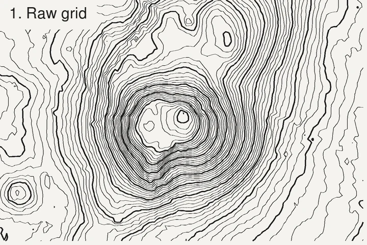
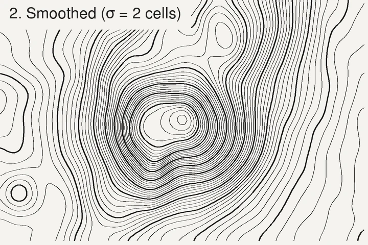
- Smooth the elevation grid with a Gaussian filter (standard deviation σ = 2 cells of the grid we read). Without it, contours on gentle ground follow the grid as a 90° staircase.
- Trace the contours at each level with the marching squares algorithm, as implemented in scikit-image (van der Walt et al., 2014).
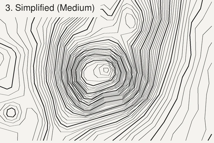
- Simplify and round the lines with the Douglas–Peucker algorithm (Douglas & Peucker, 1973), as implemented in Shapely, then round the corners, and drop lines shorter than the minimum length you set.
- Render to SVG, PNG, GeoJSON or DXF. Raster reading is done with rasterio, which builds on GDAL.
Where accuracy is lost
- The source data. A contour can’t beat the model under it: metres to tens of metres vertically for the global 30 m models, depending on slope and forest cover (GEDTM30’s authors report an RMSE of 10.7 m against GNSS stations worldwide; Ho et al., 2025), and about 10 cm for good national lidar on open ground. See global models compared.
- The smoothing. σ = 2 cells is a standard deviation of 60 m on 30 m data, and 10 m on 5 m data (for large zones the grid we read is coarser than the source, so σ grows with it). Features narrower than a few cells (a ditch, a narrow ridge, a small quarry) are softened, and sharp summits or gully bottoms can lose a few metres. That’s the price of clean lines; it’s the same trade-off any cartographer makes when generalising contours.
- Simplification and rounding move lines horizontally by up to the tolerance used: about 6, 15 or 24 m for the Low, Medium and High settings, whatever the data. Pro exports can turn simplification off.
- Minimum length removes small closed loops: tiny knolls and hollows disappear by design.
- The date of the data. Global models date from 2000 to 2015; national lidar from the year it was flown. Anything built or dug since is not in the contours.
If you need contours that keep every feature of the data, export the raw elevation model
from its publisher and contour it with GDAL (gdal_contour -i 1 dem.tif contours.gpkg), with
no smoothing. You’ll get the noise too, but nothing hidden.
How these pages are checked
The elevation figures, contours and comparisons on these pages are computed from the elevation data itself, with the same pipeline as the app. Every figure and link is checked against its source (the publisher’s documentation, a standard or a peer-reviewed paper); the sources are listed under References at the bottom of each page, and the date of that check is shown at the top.
Spotted a mistake? Open an issue on GitHub.
References
- van der Walt, S., Schönberger, J. L., Nunez-Iglesias, J., Boulogne, F., Warner, J. D., Yager, N., Gouillart, E., Yu, T. & the scikit-image contributors (2014). scikit-image: image processing in Python. PeerJ 2, e453. doi:10.7717/peerj.453
- Douglas, D. H. & Peucker, T. K. (1973). Algorithms for the reduction of the number of points required to represent a digitized line or its caricature. Cartographica 10(2), 112–122. doi:10.3138/FM57-6770-U75U-7727
- Ho, Y.-F., Grohmann, C. H., Lindsay, J., Reuter, H. I., Parente, L., Witjes, M. & Hengl, T. (2025). GEDTM30: global ensemble digital terrain model at 30 m and derived multiscale terrain variables. PeerJ 13, e19673. doi:10.7717/peerj.19673
Last updated 5 November 2026