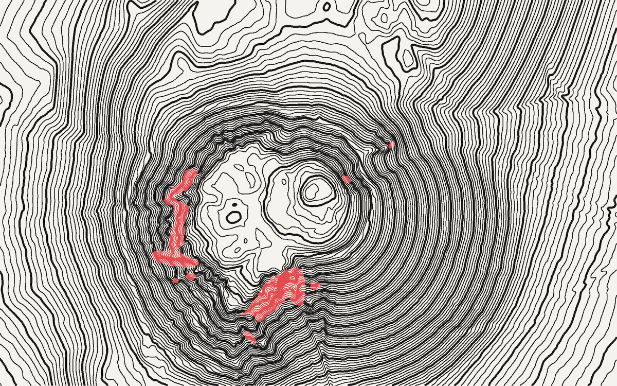
The contour interval is the height difference between two neighbouring lines. Pick it too small and steep slopes turn into a solid black smear, while flat ground fills with lines that trace the noise in your data. Pick it too large and the hills you wanted to show disappear.
New to contour lines? Start with what a contour map is, or how to draw contour lines by hand.
There is no single right number, but three quick checks get you there. Run them in order: each one sets a limit, and the interval you want sits between them.
1. The data sets the floor
A contour can’t be more precise than the elevation model under it. If your data is accurate to ±2 m, 1 m contours are drawing errors, not terrain.
The rule that mapping agencies have used since 1947 comes from the US National Map Accuracy Standards: no more than 10% of the elevations tested may be off by more than half the contour interval. Turned around, and with errors expressed as an RMSE (root-mean-square error), as today’s standards do (ASPRS, 2015), that gives:
smallest interval ≈ 3.3 × the vertical RMSE of your data
Half the interval has to cover 90% of the errors, which is 1.6449 × RMSE when errors are normally distributed, so the interval is 2 × 1.6449 ≈ 3.29 × RMSE. That’s the conversion the US federal accuracy standard gives between NMAS and RMSE (FGDC, 1998, Appendix 3-D). If your data sheet gives a 90% error (LE90) instead of an RMSE, the rule is simply interval ≥ 2 × LE90.
| Data | Vertical accuracy | Smallest interval by this rule |
|---|---|---|
| Airborne lidar DTM, open ground | RMSE ≤ 0.10 m (USGS quality level 2 and better) | 0.5 m |
| Lidar DTM under forest, or older lidar | RMSE 0.2–0.5 m | 1–2 m |
| National photogrammetric DTM | RMSE 0.5–1.5 m | 2–5 m |
| Copernicus GLO-30 and models built on it | under 4 m at 90% (spec), i.e. RMSE ≈ 2.4 m; worse under forest and on steep slopes | about 10 m |
| SRTM | 5.6–9 m at 90%, depending on the continent (Rodríguez et al., 2006) | 20 m and up |
Two nuances matter in practice:
- The rule is about reading heights. It tells you which interval lets a reader trust the number on a line. A constant offset (say the whole model sits 2 m too high) moves every line by the same amount and doesn’t change the shape of the drawing. So a designer can go finer than the floor to show the texture of the land, as long as nobody reads the lines as surveyed heights.
- Resolution matters as well as accuracy. A 30 m grid cannot show a feature narrower than about two or three cells, whatever the interval. And a comparison of ten global models against lidar found that none does well on low, flat terrain (Guth et al., 2024): there, fine intervals mostly draw noise.
See the global models compared and the French and US pages for the accuracy of each dataset.
2. The steepest slope sets the ceiling of density
On your steepest slope, the lines bunch together. On paper, the gap between two lines is:
gap on paper = interval ÷ tan(slope) ÷ scale
How close can printed lines get before they merge? Classic cartography handbooks give 0.2 mm between contour lines (Töpfer, 1974) to 0.25 mm between parallel lines (Swiss Society of Cartography, 1980). A review of these guidelines in a recent thesis on minimum map dimensions notes that most of them were never tested experimentally (Ledermann, 2023, which cites both), so treat them as rules of thumb for good print and good eyesight. We use 0.2 mm. Here is the gap, in millimetres on paper, for common scales and slopes:
| Scale | Interval | 10° slope | 30° slope | 45° slope |
|---|---|---|---|---|
| 1:10,000 | 2 m | 1.13 | 0.35 | 0.20 |
| 1:10,000 | 5 m | 2.84 | 0.87 | 0.50 |
| 1:25,000 | 5 m | 1.13 | 0.35 | 0.20 |
| 1:25,000 | 10 m | 2.27 | 0.69 | 0.40 |
| 1:50,000 | 10 m | 1.13 | 0.35 | 0.20 |
| 1:50,000 | 20 m | 2.27 | 0.69 | 0.40 |
| 1:100,000 | 20 m | 1.13 | 0.35 | 0.20 |
| 1:100,000 | 50 m | 2.84 | 0.87 | 0.50 |
Here is what that looks like on real terrain: the Puy de Dôme, a volcanic cone rising out of a gentle plateau. On its flanks, half the slopes are steeper than about 30°, and one in ten steeper than 40° (measured on IGN’s RGE ALTI at 5 m). Two settings move the lines apart: a larger interval, or a smaller area on the same sheet. A smaller interval does the opposite. Try both and watch the red, where the lines would run together in print:
Reading the table: at 1:25,000, a 5 m interval is fine on 30° slopes but merges on 45° ones. That’s why mountain maps either take a larger interval or let cliffs be drawn as rock symbols instead of contours, as Eduard Imhof describes in Cartographic Relief Presentation, still the reference on the subject (Imhof, 1982).
For a screen or a poster without a fixed scale, the same logic applies in pixels: in an export 4000 px wide, keep at least 2–3 px between lines on the steepest slope you care about.
3. The relief sets the number of lines
Divide the height range of your area by the interval: that’s how many contour levels you’ll draw. These ranges are our own rules of thumb from making maps, not a standard:
- Under ~10 levels: the landform barely reads. Fine for a flat site plan, thin for a map.
- 20–60 levels: the comfortable range for most maps and posters.
- Well over 100: dense and textural. Good for an art print, heavy for a working map.
Example: a valley from 500 m to 2,400 m is 1,900 m of relief. A 50 m interval gives 38 levels; 20 m gives 95.
Index contours
Make every 5th line an index contour, drawn thicker and labelled, as on USGS and most national topographic maps. With a 10 m interval, that’s every 50 m; with 20 m, every 100 m (reading them on an existing map: how to calculate a contour interval). Every 4th line also works for intervals like 25 m (index every 100 m). The point is that the index values are round numbers a reader can count from.
Label index contours so the numbers read uphill, and break the line under the label rather than writing on top of it.
Where national maps land
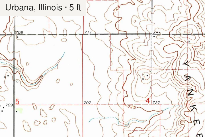
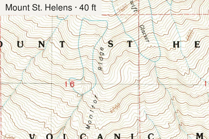
As a sanity check: USGS chooses the interval quadrangle by quadrangle, depending on the scale and the terrain. Its 1:100,000 maps use 5, 10, 20 or 50 m depending on relief (USGS), and its 1:24,000 maps range from 5 or 10 ft on flat ground to 40 ft and more in the mountains. Most 1:25,000 hiking maps in Europe sit between 5 and 20 m. If your choice is far outside that range at a similar scale, one of the three checks above probably explains why.
Doing it
- QGIS / GDAL: Raster › Extraction › Contour with your interval, then a rule-based
style where
"ELEV" % 50 = 0draws the index lines. Our QGIS walkthrough covers it step by step. - TopoLines: the interval and index contours are set in line styling, labels in cartographic options.
References
- U.S. Bureau of the Budget (1947). United States National Map Accuracy Standards. reproduced in USGS, Map Accuracy (National Mapping Program fact sheet).
- Federal Geographic Data Committee (1998). Geospatial Positioning Accuracy Standards, Part 3: National Standard for Spatial Data Accuracy (FGDC-STD-007.3-1998). FGDC, Reston, Virginia (Appendix 3-D: relationship with NMAS).
- American Society for Photogrammetry and Remote Sensing (ASPRS) (2015). ASPRS Positional Accuracy Standards for Digital Geospatial Data (Edition 1, Version 1.0). Photogrammetric Engineering & Remote Sensing 81(3), A1–A26. doi:10.14358/PERS.81.3.A1-A26
- U.S. Geological Survey (2024). Topographic data quality levels (QLs). 3D Elevation Program.
- Rodríguez, E., Morris, C. S. & Belz, J. E. (2006). A global assessment of the SRTM performance. Photogrammetric Engineering & Remote Sensing 72(3), 249–260. doi:10.14358/PERS.72.3.249
- Guth, P. L., Trevisani, S., Grohmann, C. H., Lindsay, J., Gesch, D., Hawker, L. & Bielski, C. (2024). Ranking of 10 global one-arc-second DEMs reveals limitations in terrain morphology representation. Remote Sensing 16(17), 3273. doi:10.3390/rs16173273
- Ledermann, F. (2023). Empirical assessment of minimum dimensions for cartographic symbology on smartphone displays. Doctoral thesis, TU Wien. doi:10.34726/hss.2023.53486
- Imhof, E. (1982). Cartographic Relief Presentation (ed. H. J. Steward; reissued by Esri Press, 2007). Walter de Gruyter, Berlin.
- U.S. Geological Survey (1994). USGS Maps. General Interest Publication.
Last updated 5 November 2026