# How contours are traced
> The method behind every TopoLines trace: marching squares on the elevation grid, smoothing sized to the data, a simplification tolerance in ground metres with no crossing lines, terrain below sea level, depressions, the coast, and the known limits. With the benchmark figures and the papers it rests on.
Source: https://www.topolines.app/docs/contour-engine · TopoLines docs · updated 2026-11-15
Every TopoLines map, Lines or Points, PNG, SVG, GeoJSON or DXF, is traced by the same
engine on our server. This page describes what it does, in order, and why. It gives the
principles and the measured results; the exact tuning constants stay internal. The numbers
quoted come from a benchmark of real and synthetic terrain, described in full in
[What the tracer does to a contour line](https://www.topolines.app/atlas/contour-tracing-accuracy).
## In short
Measured on the benchmark zones and sources described [below](#benchmark-results):
- **Smoothing follows the grid served.** On GEDTM30, crests lose 1.0 to 2.6 m on average,
against 15 to 31 m with the previous fixed width.
- **The tolerance is in ground metres, the same north–south and east–west.** The largest
displacement reaches the step's tolerance and no more, from 36° N to 61° N.
- **All lines are simplified as one geometry.** 0 crossings between levels and 0
self-intersections on every zone tested.
- **Depressions and land below sea level are kept.** Badwater Basin gets its −25, −50 and
−75 m contours.
## The steps
Every trace goes through the same chain, on our server. Each step is described below.
1. **Read the elevation grid** for the zone: GEDTM30 by default, a national lidar model for
HD exports where one exists, or your own GeoTIFF ([sources](#data-sources)).
2. **Find the sea**, and keep everything else as land, including land below 0 m.
3. **Smooth the grid** lightly, by an amount set by the size of its cells.
4. **Trace each level** with marching squares.
5. **Cut the lines at the coast.**
6. **Simplify all lines together**, with a tolerance in metres on the ground.
7. **Drop the shortest lines**, if you asked for it.
8. **Render or export.** GeoJSON and DXF carry the traced coordinates themselves, with
their elevation; only the PNG is rounded to pixels.
## Tracing: marching squares
Each level is traced with the marching squares algorithm as implemented in
[scikit-image](https://scikit-image.org/)
([van der Walt et al., 2014](https://doi.org/10.7717/peerj.453)). Every height is placed at
the centre of its grid cell, and the crossing point on each cell edge is found by linear
interpolation between the two corners. A raw trace therefore has one vertex per cell edge
it crosses, and the line is where the grid says the level is, to within that linear
interpolation between two samples: nothing tells the tracer what the ground does between
them.
Two things follow from tracing a grid:
- **Lines of different levels do not cross on the raw trace.** This is a property of the
model: every line is a level of the same interpolated surface, and a point of that surface
has one height, so it cannot lie on two levels. Marching squares keeps it by applying the
same rule at every level, saddles included. Checked on the benchmark: 0 crossings between
levels on every zone and source tested.
- **Saddle cells are ambiguous.** When the four corners of a cell alternate above and below
the level, two ways of joining the line are both valid. TopoLines uses the fixed rule of
scikit-image's `find_contours` with low connectivity: the two corners below the level are
joined across the saddle. The asymptotic decider of
[Nielson & Hamann (1991)](https://doi.org/10.1109/visual.1991.175782), which picks the join
from the interpolated value at the saddle, is not used. What that implies: at a saddle
cell, the line can occasionally take the other of the two valid joins, so two lines that
meet at a pass may be connected differently. It never makes two levels cross. On the
benchmark's synthetic saddle every vertex lies within half a cell of the exact curve; that
is a result on that one test terrain, not a general guarantee.
## Smoothing, sized to the data
A grid is noisy at the scale of its own cells ([Fisher & Tate, 2006](https://doi.org/10.1191/0309133306pp492ra)),
and marching squares turns that noise into a zig-zag, cell by cell. A light Gaussian
smoothing removes it before tracing. Two rules set its width:
- **It is set in metres on the ground and is the same in every direction.** Global grids
are laid out in degrees, so their cells are narrower east–west than north–south (half as
wide at 60° N). A width counted in cells smoothed twice as far north–south. The width is
now chosen in metres, then converted into a number of cells separately for each axis, from
the real ground size of the cells on that axis at the zone's latitude. The blur is
therefore the same distance on the ground in both directions, on a grid in degrees.
- **It follows the cell size of the grid actually served, and depends on the source.**
GEDTM30 has already been filtered by its authors (an adaptive filter and a bilateral
filter, [Ho et al., 2025](https://doi.org/10.7717/peerj.19673)), so it gets a fraction of
a cell. Raw national lidar gets more, to take out the grid noise.
No single width works for every grid: what a 2 m lidar grid needs would erase the relief
of a 30 m grid, and the reverse. The smoothing is internal; there is no setting for it.
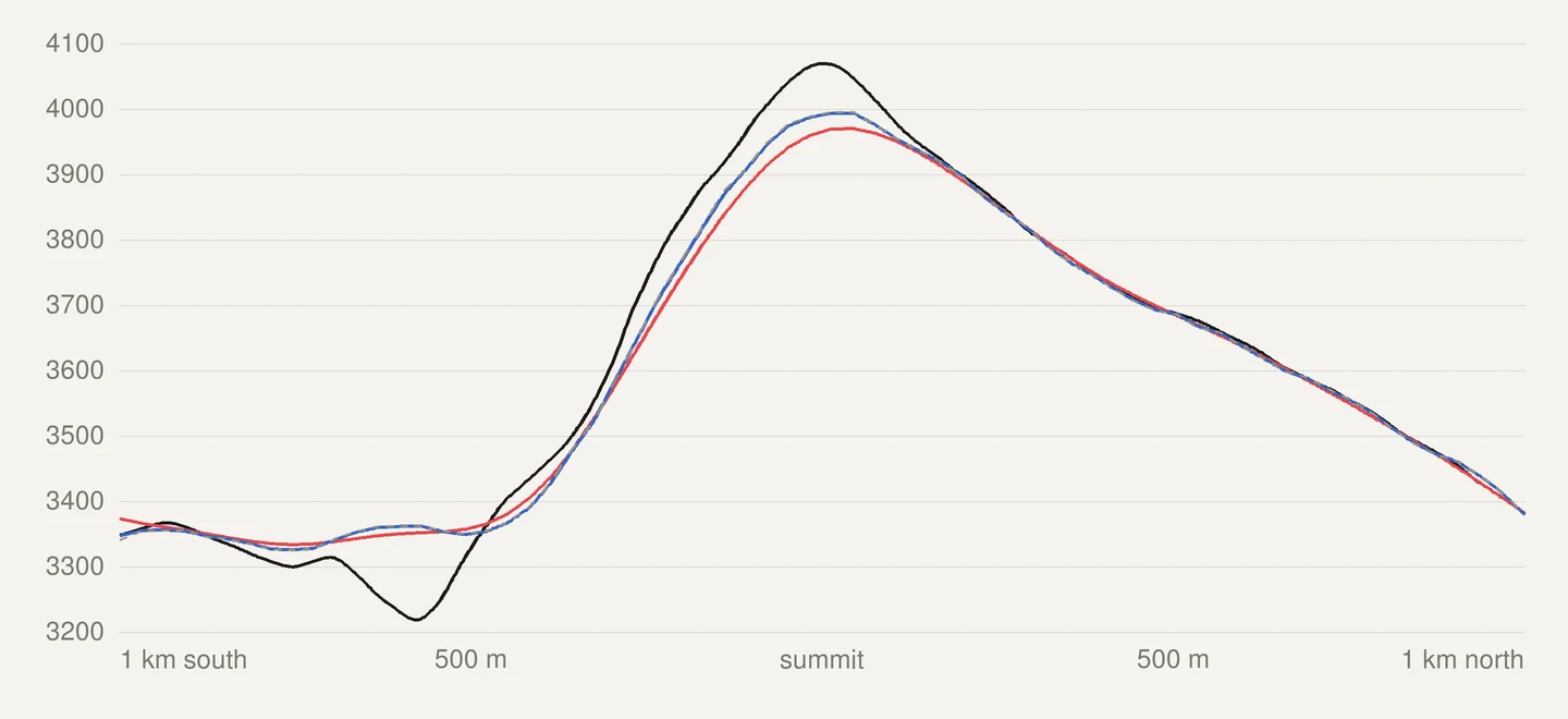
Effect measured on the benchmark, against the previous fixed width of two cells (until
v2.55):
| | Previous smoothing | Current smoothing |
| --- | --- | --- |
| GEDTM30 crests, mean change | −15 to −31 m | −1.0 to −2.6 m |
| GEDTM30 valley floors, mean change | +12 to +26 m | +1.0 to +2.9 m |
| Raw trace more than half an interval away from the published grid, share of its length (five relief zones) | 0.14 to 15.6 % | ≤ 0.01 % |
| Small closed depressions kept (Girdwood, Alaska, 75 in the raw grid) | 3 | 37 |
Two adaptive methods from the literature were tested on the same benchmark and not
retained: the TPI-weighted blend of [Kettunen et al. (2017)](https://doi.org/10.1080/23729333.2017.1300998)
and the feature-preserving smoothing of [Lindsay et al. (2019)](https://doi.org/10.3390/rs11161926).
The reasons are in the [Atlas article](https://www.topolines.app/atlas/contour-tracing-accuracy#what-was-tried-and-dropped).
## Simplification
The raw trace has one vertex per cell edge: hundreds of thousands of points on an HD zone.
**Simplification** in the Settings panel removes the points that do not change the shape of
the line.
### A tolerance in metres, the same in every direction
Each step is the **largest distance a line may move on the ground**, east–west and
north–south alike:
| Step | Tolerance | Notes |
| --- | --- | --- |
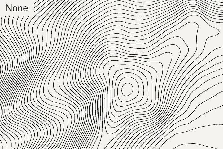
| **None** | — | The raw trace (Pro). |
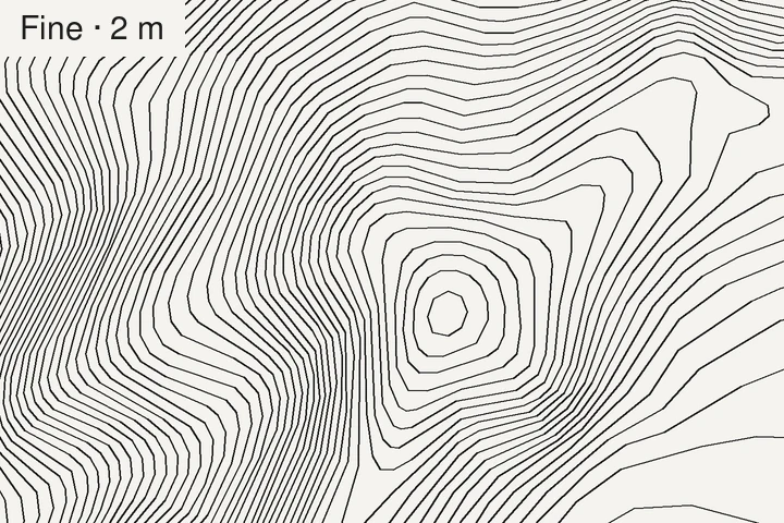
| **Fine · 2 m** | 2 m | Removes the cell-by-cell zig-zag of a lidar trace. |
| **Low · 6 m** | 6 m | |
| **Medium · 15 m** | 15 m | Default. |
| **High · 24 m** | 24 m | Lightest files. |
The algorithm underneath is Douglas–Peucker
([Douglas & Peucker, 1973](https://doi.org/10.3138/fm57-6770-u75u-7727)). It guarantees the
bound: the vertices it keeps are vertices of the raw trace, and every vertex it removes lies
within the tolerance of the shortcut that replaces it, so the symmetric Hausdorff distance
between a simplified line and its raw trace cannot exceed the tolerance. Measured on the
benchmark, the maximum reaches the tolerance, to rounding, at every latitude tested
(36° N to 61° N). The distances are computed on a local metric scale at the zone's
latitude, which is within ±0.35 % of a projected distance on zones up to 45 km across.
### Lines do not cross after simplification
Simplifying each line on its own lets a shortcut on one line jump over its neighbour on a
steep slope. Using a "topology-preserving" option line by line does not prevent it: that
option only checks the line against itself. In a synthetic trial it removed none of the
crossings.
TopoLines passes **all the contours of the zone and the coastline as one geometry**, a
single multi-line collection, to the `TopologyPreservingSimplifier` of
[GEOS](https://libgeos.org/) (GEOS 3.13.1 through [Shapely](https://shapely.readthedocs.io/)
2.1.2). Within a collection, GEOS refuses any shortcut that would cut another segment of
the collection, not only a segment of the same line, and any that would turn a ring inside
out. This is the constraint of [Saalfeld (1999)](https://doi.org/10.1559/152304099782424901)
applied to the whole set. Because the coastline is part of the set, no contour can be
simplified across it.
Three things, kept apart:
- **What the model gives:** no two levels cross on the raw trace (above).
- **What the joint simplification preserves:** it removes a vertex only if no crossing and
no self-intersection appears, so a set without crossings stays without crossings.
- **What was measured:** 0 crossings between levels and 0 self-intersections on every zone
and source tested, at every step (High used to leave up to 18 crossing pairs on steep
lidar zones), for between 0 and 3 % more points depending on the zone.
### Recommended
After a trace, a **Recommended** tag marks the step that suits the zone. It is a hint;
nothing is selected for you. It weighs three things:
- **The cell size of the grid actually served.** Below a fraction of a cell, simplifying
removes no information the data holds.
- **The median spacing between neighbouring contours**, from the interval and the median
slope. The tolerance must stay well below that spacing, so that a simplified line keeps
clear of its neighbours: rule R4 of [Bayer et al. (2023)](https://doi.org/10.1080/13658816.2023.2193969),
and the displacement that a vertical error allows on a slope, as used by
[Miller (2024)](https://doi.org/10.5311/josis.2024.28.245).
- **How many points the trace would carry**, so that a large lidar zone stays light enough
to open in a design tool.
In practice it lands on Medium on GEDTM30, on Fine on 5 m lidar, and one step lower on
steep terrain with a fine interval.
## Minimum contour length
**Min. contour length** drops lines shorter than the chosen length, after simplification.
**Auto** (the default) picks the length from the terrain: it compares the lines with the
median spacing between contours, then backs off so it never removes a large share of the
traced length. On a Dutch polder at 5 m it removes the swarm of tiny loops left by
centimetre-scale relief (1,294 closed loops down to 360); in the mountains it keeps 99 % or
more of the length. Removing short lines is also the last step of
[Kettunen et al. (2017)](https://doi.org/10.1080/23729333.2017.1300998). See
[cartographic options](https://www.topolines.app/docs/cartographic-options#minimum-contour-length).
## Sea, land below 0 m and depressions
- **Land below sea level is traced.** Death Valley's Badwater Basin (−85 m) gets its −25,
−50 and −75 m contours, and a Dutch polder its contours down to −10 m. Earlier versions
treated every height at or below 0 m as sea.
- **The sea.** The data producers flatten water into a constant surface at sea level, or
leave it empty. TopoLines treats that flat surface as sea where it reaches the open
water, and cuts the contours along the
[OpenStreetMap coastline](https://wiki.openstreetmap.org/wiki/Coastline) when it is
available, so the shore is drawn where it is mapped rather than where the model happens
to cross 0 m.
- **Depressions.** Marching squares orients every line with the lower ground on one fixed
side, so a closed ring around a pit is recognised exactly from its direction, and marked
with inward ticks if you show depression contours. A ring along a plateau sitting exactly
at the level is not a depression. Checked against the previous method on 781 closed rings from
the real zones: the 55 disagreements were all small rings, and every one large enough to
sample is lower inside.
## Data sources
The grid behind your zone is named in **Map info** and, with its credit, in the metadata
of every export. The benchmark used these three, each the work of public institutions or
researchers who chose to publish it openly:
- **[GEDTM30](https://codeberg.org/openlandmap/GEDTM30) v1.2**, the Global Ensemble Digital
Terrain Model at 30 m, by Yu-Feng Ho, Tom Hengl and colleagues at
[OpenGeoHub](https://opengeohub.org/) ([Ho et al., 2025](https://doi.org/10.7717/peerj.19673);
data: [Ho & Hengl, 2026, Zenodo](https://doi.org/10.5281/zenodo.18887460)), CC BY 4.0,
read through [OpenTopography](https://opentopography.org/). A bare-earth model trained on
satellite lidar, the default everywhere.
- **[RGE ALTI®](https://cartes.gouv.fr/rechercher-une-donnee/dataset/IGNF_RGE-ALTI)** by
[IGN](https://www.ign.fr/), the French national 1 m terrain model, Etalab Open Licence 2.0.
- **[3DEP](https://www.usgs.gov/3d-elevation-program)**, the 3D Elevation Program of the
U.S. Geological Survey, public domain.
Every other national model (Austria, England, Germany, Italy, Spain, Switzerland) is listed
with its publisher and licence in [Datasets](https://www.topolines.app/docs/datasets).
## Known limits
- **The data comes first.** A contour cannot be more accurate than the grid. A height error
*h* on a slope θ moves a contour sideways by *h* / tan θ: a 5 m error is 9 m on a 30° slope
and 95 m on a 3° slope ([Miller, 2024](https://doi.org/10.5311/josis.2024.28.245) uses the
same relation the other way round). Flat ground is where lines are least reliable. More in
[how far off a contour line can be](https://www.topolines.app/atlas/contour-line-uncertainty) and
[what DEM error does to a contour line](https://www.topolines.app/atlas/dem-error-contour-lines).
- **The wobble in None is real.** On 2 m lidar, a raw trace that still trembles after
smoothing is following rocks, scree and small steps in the model, not grid noise. Fine ·
2 m is the step for it.
- **Flat ground at a fine interval** draws many small loops around relief of a few
decimetres on a 30 m model. They are in the data; Auto minimum length clears most of them.
Not every closed depression in a DEM is real
([Lindsay & Creed, 2006](https://doi.org/10.1016/j.cageo.2005.11.002)).
- **The coast.** Where the coastline cannot be fetched, the sea is cut along the model's
own water surface instead, which is coarser. Lagoons and very low coastal plains (the
Camargue) are the hardest case: the benchmark cannot always tell shallow water from land
just below 0 m.
- **Smoothing has a cost.** A ditch or a ridge narrower than a few cells is softened, and a
sharp summit loses a little height (1 to 3 m on GEDTM30 crests on the benchmark).
- **Not survey data.** See [accuracy and limits](https://www.topolines.app/atlas/accuracy-and-limits) for what
contours from open data must not be used for.
## Benchmark results
The engine is checked against two sets: the synthetic one runs with the test suite on every
change, the real zones are re-measured at each change to the engine. The results below hold
for the zones and sources listed here, and only for them.
- **Synthetic terrain with a known answer**: a Gaussian hill at 0, 45, 60 and 70° of
latitude, a saddle, a ridge and valley, a noisy steep slope, a tilted plane, a basin below
sea level, a polder behind a dyke. On these terrains the traced rings of the hill match
the analytic radius to within half a cell, and the tilted plane is exact to 0.01 cell at
every latitude.
- **Six real zones**, each traced on GEDTM30 and on the national lidar where there is one:
the Calanques, the Écrins, the Camargue, Badwater Basin, the Zuidplaspolder and Girdwood
(Alaska, 61° N), plus the Aiguille du Midi on IGN 2 m for the smoothing.
| Measure (real zones) | Before the 2026 engine pass | Now |
| --- | --- | --- |
| Crossing pairs between levels, High | up to 18 | 0 |
| Self-intersecting lines, any step | up to 9 | 0 |
| Largest line displacement, Medium at 61° N | 30.6 m north–south | 15.0 m (the tolerance) |
| Badwater Basin area treated as sea | 51.9 % | 0 % |
| Points left by Fine · 2 m on 5 m lidar | (no such step) | 7 to 15 % of the raw trace |
A benchmark output: 2 km north–south through the Barre des Écrins summit. Black: IGN RGE ALTI 5 m. Grey dashes: GEDTM30 as published, almost hidden under the blue. Blue: GEDTM30 with the current smoothing. Red: with the previous one. At the summit the previous smoothing took 25 m off the published grid, the current one 1.4 m.Engine output, 600 × 400 m below the Aiguille du Midi, IGN RGE ALTI 2 m, every 10 m. Left: None. Right: Fine · 2 m. Over the whole 3.9 × 3.3 km zone: 597,267 points against 25,028.
### How the figures are measured
- **Crossings:** pairs of contours of different levels that touch or cross, tested with an
exact geometric predicate. The coastline is excluded; auxiliary contours are included.
- **Self-intersections:** lines that cross themselves.
- **Hausdorff distance:** symmetric, in metres, between each simplified line and the same
line before simplification, after the coast cut.
- **Raw trace more than half an interval away:** the unsimplified trace is sampled every
half cell and each sample's height is read, by bilinear interpolation, on the grid as
published (before any smoothing). The figure is the share of samples, so of the line's
length, where that height differs from the contour's level by more than half the
interval.
- **Crests and valley floors:** the mean change in height (smoothed minus published) over
the 2 % of cells that stand highest, and the 2 % that sit lowest, relative to the mean of
their surroundings within about 100 m.
- **Points:** vertices of the delivered trace; "between 0 and 3 % more" is the range over
the zones, not an average.
Zone by zone figures and the full method are in the Atlas:
[What the tracer does to a contour line](https://www.topolines.app/atlas/contour-tracing-accuracy).
### What the benchmark does not cover
Six zones and three sources cannot cover every terrain. Not tested: karst, dune fields,
volcanic terrain, dense urban centres, large ice caps (glaciers only appear in passing, in
the Écrins and at the Aiguille du Midi), latitudes beyond 61° N, and grids with strong
artefacts such as voids, stripes or tile seams. The OpenStreetMap coastline was not tested
on real zones either (see [the Atlas article](https://www.topolines.app/atlas/contour-tracing-accuracy#what-is-still-open)).
### Reproducing it
The benchmark zones are listed with their coordinates in the Atlas article, and all three
sources are open. Software: scikit-image 0.25.2 (marching squares), Shapely 2.1.2 on GEOS
3.13.1 (simplification), Python 3.12. The parameters are published as families, with the
criteria they were chosen on; their values are not:
- **Smoothing:** a Gaussian whose width is a multiple of the served cell size, with one
multiple for grids already filtered at the source and a larger one for raw lidar.
Chosen on, in order: the vertical gap between the trace and the published grid, then the
height kept on crests, valley floors and depressions, then crossings, displacement, the
cell-by-cell zig-zag, and time and memory.
- **Recommended:** the largest step under a bound set by a fraction of the cell size, with
a floor, and by a fraction of the median contour spacing, moved one step up when the
point count would exceed a budget. Chosen to land on Medium on GEDTM30 and Fine on 5 m
lidar, and to go lower on steep terrain at a fine interval.
- **Auto minimum length:** the largest step under the median contour spacing, reduced while
it would remove more than a set share of the traced length. Chosen to clear plains of
small loops while keeping mountain zones whole.
## References
- Bayer, T., Kolingerová, I., Čelonk, M. & Lysák, J. (2023). Simplification of contour
lines, based on axial splines, with high-quality results. *IJGIS* 37(7), 1520–1554.
[doi:10.1080/13658816.2023.2193969](https://doi.org/10.1080/13658816.2023.2193969)
- Douglas, D. H. & Peucker, T. K. (1973). Algorithms for the reduction of the number of
points required to represent a digitized line or its caricature. *Cartographica* 10(2),
112–122. [doi:10.3138/fm57-6770-u75u-7727](https://doi.org/10.3138/fm57-6770-u75u-7727)
- Fisher, P. F. & Tate, N. J. (2006). Causes and consequences of error in digital elevation
models. *Progress in Physical Geography* 30(4), 467–489.
[doi:10.1191/0309133306pp492ra](https://doi.org/10.1191/0309133306pp492ra)
- Ho, Y.-F., Grohmann, C. H., Lindsay, J., Reuter, H. I., Parente, L., Witjes, M. & Hengl,
T. (2025). GEDTM30: global ensemble digital terrain model at 30 m and derived multiscale
terrain variables. *PeerJ* 13, e19673.
[doi:10.7717/peerj.19673](https://doi.org/10.7717/peerj.19673)
- Kettunen, P., Koski, C. & Oksanen, J. (2017). A design of contour generation for
topographic maps with adaptive DEM smoothing. *International Journal of Cartography*
3(1), 19–30. [doi:10.1080/23729333.2017.1300998](https://doi.org/10.1080/23729333.2017.1300998)
- Lindsay, J. B. & Creed, I. F. (2006). Distinguishing actual and artefact depressions in
digital elevation data. *Computers & Geosciences* 32(8), 1192–1204.
[doi:10.1016/j.cageo.2005.11.002](https://doi.org/10.1016/j.cageo.2005.11.002)
- Lindsay, J. B., Francioni, A. & Cockburn, J. M. H. (2019). LiDAR DEM smoothing and the
preservation of drainage features. *Remote Sensing* 11(16), 1926.
[doi:10.3390/rs11161926](https://doi.org/10.3390/rs11161926)
- Miller, S. (2024). Locally adjusted curve approximation smoothing of contour polylines.
*JOSIS* 28, 3–73. [doi:10.5311/josis.2024.28.245](https://doi.org/10.5311/josis.2024.28.245)
- Nielson, G. & Hamann, B. (1991). The asymptotic decider: resolving the ambiguity in
marching cubes. *IEEE Visualization '91*, 83–91.
[doi:10.1109/visual.1991.175782](https://doi.org/10.1109/visual.1991.175782)
- Saalfeld, A. (1999). Topologically consistent line simplification with the
Douglas-Peucker algorithm. *Cartography and Geographic Information Science* 26(1), 7–18.
[doi:10.1559/152304099782424901](https://doi.org/10.1559/152304099782424901)
- van der Walt, S., Schönberger, J. L., Nunez-Iglesias, J., Boulogne, F., Warner, J. D.,
Yager, N., Gouillart, E., Yu, T. & the scikit-image contributors (2014). scikit-image:
image processing in Python. *PeerJ* 2, e453.
[doi:10.7717/peerj.453](https://doi.org/10.7717/peerj.453)